How to put and use the pi number in microsoft excel data table? Step by step guide

Today, worldwide, Excel is considered one of the most useful office programs, since it consists of an arrangement of rows and columns divided by boxes that simplify the preparation, modification and handling of spreadsheets . As a result, it is essential for organizational, accounting, financial, and scheduling tasks .

In this sense, in addition to facilitating the organization and tabulation of any type of information, this program stands out for allowing the insertion of numerical data in order to store and interpret them for study. Taking into account that, it provides numerous functions with which it is possible to carry out any kind of calculation .

Therefore, through Microsoft Excel, users have the ability to use a myriad of mathematical and trigonometric formulas to perform their tasks effectively. Therefore, it is possible to make use of the recognized PI number in any data table, without it throwing an error in the program.

What should we take into consideration when applying the PI function on a data table?

Before knowing how to use the PI function correctly in an Excel data table, it is necessary to clarify certain parameters of interest. Since, it is a representative number that cannot be used in any way in this Microsoft software . Thus, basically, the PI function in Excel is responsible for returning the mathematical constant π (3.14…), used in different equations and functions, at a global level. Like, for example, to calculate the area of ​​a circle using the usual formula for it .

However, when making use of this constant value in the Microsoft spreadsheet, it is necessary to use the term “PI”, instead of using the symbol that represents it, that is, “π” . Since, the latter will not be able to be recognized as an entry in the program and, consequently, will throw an error.

On the other hand, it is appropriate to clarify that, as in any calculator or mathematical program that supports equations, in Excel it is possible to perform any operation using the PI number . In other words, there is no limitation whatsoever to add, subtract, multiply or divide said  digit , for example. Like, to add it in certain functions that the software provides.

Steps to use the PI function and use this number in your Microsoft Excel spreadsheets

Now, you wonder  how you can use the PI function to use that number in your spreadsheets and complete your tasks satisfactorily , without getting some errors as a result.

Reason why, below, we specify each and every one of the steps to follow to handle the “π” in Excel:

• If you want to call the PI function in this program manually and directly, the first thing you have to do is find the cell in which you want to specify said mathematical number .
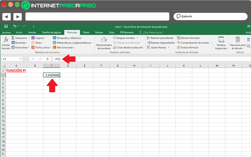
• Next, copy the following: “= PI ()” without using the quotation marks and press the Enter key; in this way, you will be able to obtain the complete π number.

• In case you want to perform a mathematical operation, you must specify it before pressing the Enter key . Once you do it, you will get the result in the established box.

Besides the manual-direct method of calling the PI function in Excel, there is also another tactic you can use .

Next, we explain how:

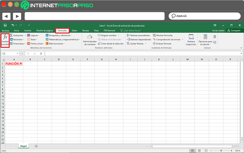
• Access a blank spreadsheet or, failing that, enter the Excel document in which you want to use the PI function .
• Now, go to the program’s ribbon and there, click on the “Formulas” tab . Then, within the group called Function Library, select the option that says “Insert function . “

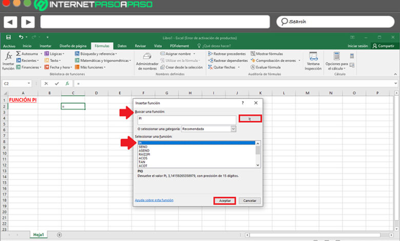
• Once this is done, a new box will appear on the screen and using it, enter the term “PI” in the Search for a function bar. To do so, click on “Go” .
• Finally, this function will appear and it is enough to select it to click on “Accept”, that way, when you confirm the action again, it will be displayed in the cell indicated at the beginning of the process . From there, you can make and edit the calculations you require.