How to hide the content of a cell in Excel easily

In this portal we want to make your life easy and for this we have published easier and more complete tutorials to handle Excel like an expert. This time we are going to talk about how to hide the content of a cell in Excel  easily or make it invisible.

This information is very useful, since there are times when you want to hide the information contained in these cells quickly and thus remain private, such as bank codes, account numbers, etc. The good thing is that said information will not stop being in these cells and at another time you can show it again.

Learn how to hide the contents of a cell in Excel

So that people who open your file cannot see the information you want to hide in certain cells, you must follow the steps described below:

1. In Microsoft Excel, open the workbook that contains the cells whose content you want to hide, or if it doesn’t start with a new workbook, and enter the data you want to hide in the cell in question.
2. You select the cell that contains the text to be hidden and make that text transparent, so you hide the content of the cell easily and the people who open the file will not see the information, as they will only see a blank cell.

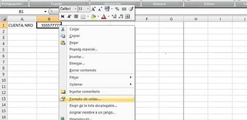
A second option is to select the cell, click the right mouse button and touch the Format Cells dialog box . You can change the cell format whenever you want , if you want to learn how to do it we already published it in an article on our blog a few days ago; But let’s continue with the example that we have taken so far:

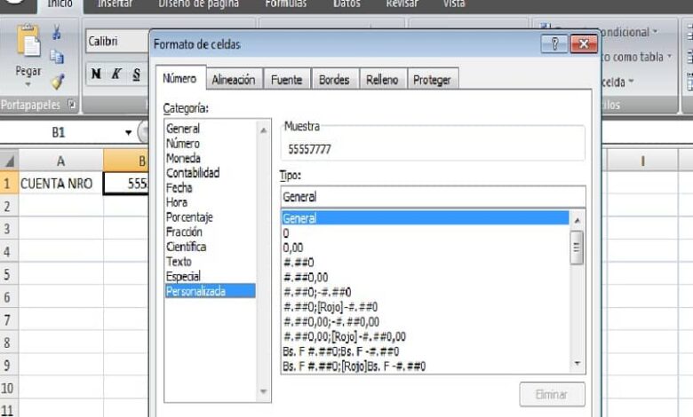
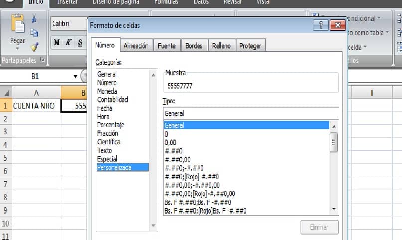
1. Once in the Cell Format dialog box, touch the Number tab and Category opens; within this you click on Custom. In General type, you eliminate General and put the semicolon symbol (;;;) three times.
2. You click OK and you will see that the text contained in the cell disappears while the Format Cells dialog box closes .

These simple steps that we have just described to hide the content of a cell in Excel easily ; It is also useful when you want the information not to be printed, having the peace of mind that the content has not disappeared from it. You will only see it in the formula bar if you click on the cell.

If you want to display the content, you can also remove the three semicolons (;;;); and put the General format back. There are also other steps to show or hide formulas in an Excel sheet.

Steps to hide content with a sheet or cell protection

Now, if you really want to hide the content of the cell and not show it in the formula bar or protect it, you must protect the spreadsheet you are working on. To do this, you must act as follows:

1. Select the cell in question and hit the Ctrl + 1 keys or enter the Format Cell dialog box .
2. Once there you touch the Protect tab. Here you select Hidden.
3. Once this is done, go to the Review tab, then in Changes you click the Protect sheet command.
4. In the section where it says Protect sheet and Contents of locked cells should be the symbol √, check or uncheck as needed.
5. If you wish, you can put a password, so you will have more security that they will not have access to the information that you want to hide.
6. Finally click OK to safely hide the content of the cell so that it is not displayed in the formula bar.

On this page we will help you handle Excel like a true expert. We can teach you, for example, how to hide an excel sheet with a macro   or how to eliminate a circular reference and many more details that will help you with this powerful and versatile Excel tool.